| Locally Optimal Control Strategy | |
 |  |
| Developing general controllers that can be applied to large classes of nonlinear systems is an ongoing goal of controls engineers. We recently used a combination of nonlinear systems analysis and optimal control to develop a routine we call the Locally Optimal Control Strategy, or LOCS. The routine consists of two pieces: (1) a nonlinear system can be approximated by a linear system about an arbitrary point in phase space and (2) the minimum energy control strategy can be equivalently expressed as a time-varying hyperellipsoid. With respect to point (1), we also know that a linear approximation of a nonlinear system is only valid within a subspace of the full phase space. With respect to point (2), this hyperellipsoid consists of all possible states of a linear system under the in uence of minimum energy control. The LOCS routine combines these two pieces by computing the intersection between the subspace where the approximate linear system is valid and the hyperellipsoid of all minimum energy controlled states. This intersection consists of all possible states that can be defined as the control goal of the minimum energy control action. With the control goal defined, that is, a terminal condition of the optimal controller, a new approximate linear model is constructed about this new point and the entire process is repeated, which justifies our description of the controller being "locally optimal". | |
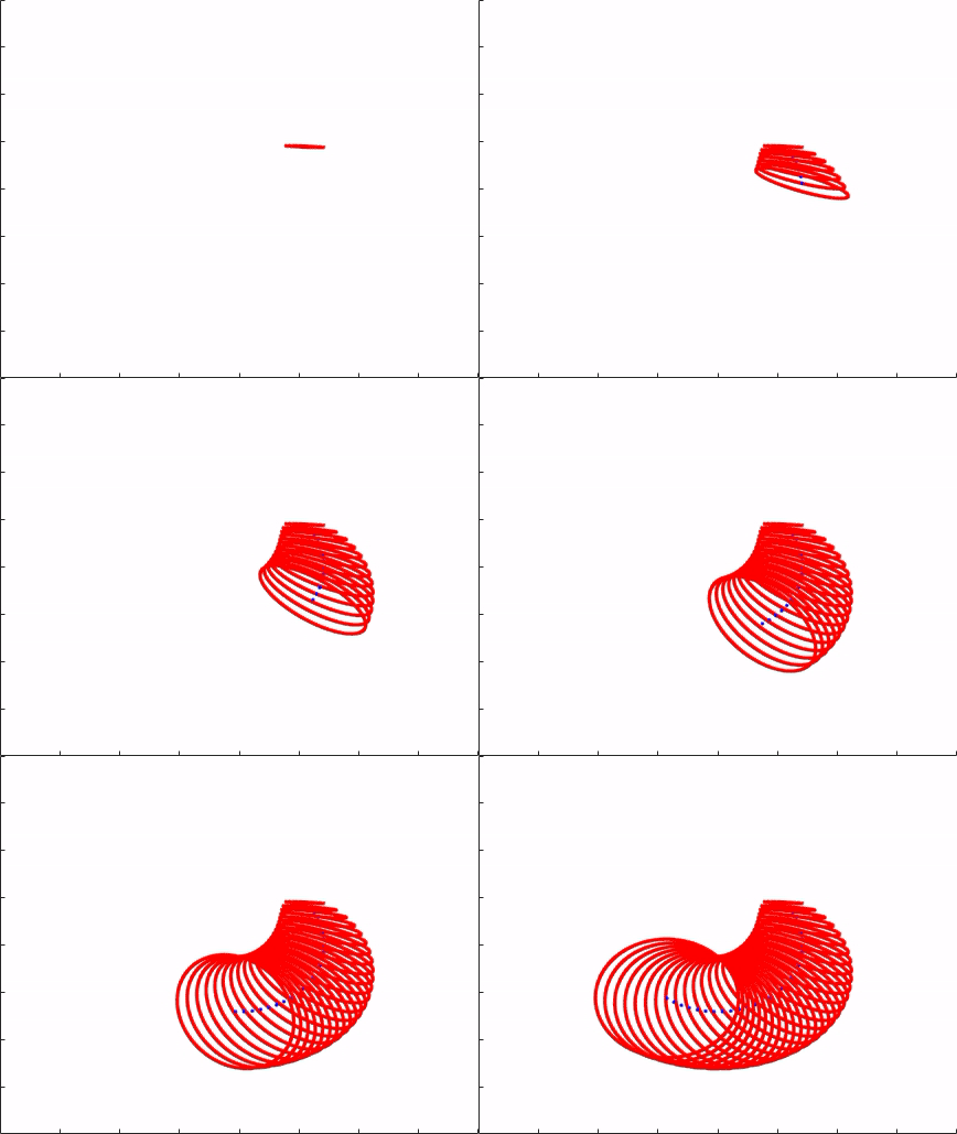
| To visualize the structure and evolution of the hyperellipsoid, we show in video 1 the hyperellipsoid
corresponding to the linear system consisting of two states, \dot{x}_1(t) = x_1(t) + u(t) \dot{x}_2(t) = -x_1(t) |
|
| This is the example that appears in Fig. 1 in the paper "Locally Optimal Control of Complex Networks" with the initial condition x_1(0) = 1 and x_2(0) = 1. | |
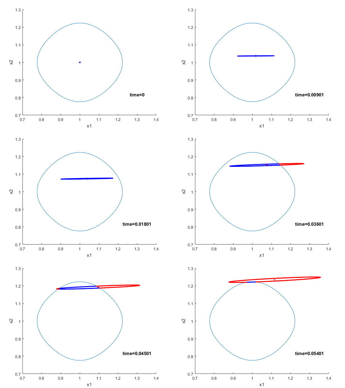
| To visualize the intersection between the valid linearized region and the hyperellipsoid, we also plot
the evolution of the hyperellipsoid corresponding to a linearized model of the nonlinear system \dot{x}_1(t) = x_1(t)x_2(t) + u(t) \dot{x}_2(t) = x_1^2(t) + x_2^2(t) |
|
| where the linearization was performed about the point x_1 = 1 and x_2 = 1. The region in which this approximate linear model is valid is also shown in video 2. | |

